
In the first part, we’ve introduced the fundamental ideas on MLP and its training method Backpropagation. In this part, let’s get started to implement those theories to come up with a keras-style MLP.
We begin with a standard import:
import numpy as np
import matplotlib.pyplot as plt
First of all, we define some activation functions and their derivatives:
def sigmoid(Z):
    return 1 / (1 + np.exp(-np.clip(Z, -250, 250)))

def relu(Z):
    return np.maximum(0, Z)

def sigmoid_bk(Z):
    sig = sigmoid(Z)
    return sig * (1 - sig)

def relu_bk(Z):
    return np.where(Z <=0, 0, 1)

act_funcs = {'sigmoid':sigmoid, 'relu':relu}
back_act = {'sigmoid': sigmoid_bk, 'relu': relu_bk}
For each layer, we need to remember the number of units, what’s the activation function, weights $W$, bias $b$, the linear combination $z$, and the output from activation function $a$. So we create a module enabling those methods:
class Layer(object):
    def __init__(self, units, activation):
        self.units = units
        self.activation = act_funcs[activation]
        self.back_act = back_act[activation]
        self.a_h = None
        self.z_h = None
        self.W = None
        self.b = None
Module Model contains the architecture of the model as well as the training processes:
class Model(object):
    def __init__(self, lr, epochs, batch_size=200, seed=123):
        self.arch = []
        self.lr = lr
        self.epochs = epochs
        self.rnd = np.random.RandomState(seed)
        self.batch_size = batch_size
        self.cost = []
        self.fit_flag = False

    def init_w(self):
        n_layers = len(self.arch)
        for i in range(1, n_layers):
            layer0 = self.arch[i-1]
            layer1 = self.arch[i]
            w_ = self.rnd.randn(layer0.units, layer1.units)
            b_ = np.zeros(layer1.units)
            layer1.W = w_
            layer1.b = b_

    def init_az(self):
        for layer in self.arch:
            layer.a_h = None
            layer.z_h = None

    def add(self, layer):
        self.arch.append(layer)

    def _compute_cost(self, y, output):
        term1 = -np.dot(y.T, np.log(output))
        term2 = np.dot((1- y).T, np.log(1 - output))
        cost = (term1 + term2)[0,0]
        dA_init = -(np.divide(y, output) - np.divide(1 - y, 1 - output))
        return cost, dA_init

    def _forward(self, layer0, layer1):
        a_h0 = layer0.a_h
        z_h1 = np.dot(a_h0, layer1.W) + layer1.b
        a_h1 = layer1.activation(z_h1)
        layer1.z_h = z_h1
        layer1.a_h = a_h1

    def _backward(self, layer0, layer1, dA):
        dW = np.dot(layer0.a_h.T, layer1.back_act(layer1.z_h) * dA)
        db = np.sum(layer1.back_act(layer1.z_h) * dA, axis=0, keepdims=True)
        dA = np.dot(layer1.back_act(layer1.z_h) * dA, layer1.W.T)
        layer1.W = layer1.W - self.lr * dW
        layer1.b = layer1.b - self.lr * db
        return dA

    def fit(self, X, y, retrain=True):
        #########################
        #init all Ws and set a_h0 = X
        #########################

        idx = [i for i in range(len(X))]
        self.rnd.shuffle(idx)
        idx = idx[:self.batch_size]
        n_layers = len(self.arch)
        self.init_w()
        if retrain:
            self.init_az()
        if X.shape[1] == self.arch[0].units:
            self.arch[0].a_h = X[idx]
        else:
            raise Exception("Input shape is not right")

        for e in range(self.epochs):
            #######################
            # forward propra
            #######################
            for i in range(1, n_layers):
                layer0 = self.arch[i - 1]
                layer1 = self.arch[i]
                self._forward(layer0, layer1)

            cost, dA_init = self._compute_cost(y[idx], self.arch[-1].a_h)
            self.cost.append(cost)
            dA = dA_init

            #######################
            # backward propra
            #######################
            for j in range(1, n_layers):
                layer0 = self.arch[-j - 1]
                layer1 = self.arch[-j]
                dA = self._backward(layer0, layer1, dA)

        self.fit_flag = True
        return self

    def predict(self, X):
        if self.fit_flag:
            n_layers = len(self.arch)
            for i in range(1, n_layers):
                layer = self.arch[i]
                Z = np.dot(X, layer.W) + layer.b
                X = layer.activation(Z)
            self.fit_flag = True
            return X
        else:
            print('The model has not been trained yet')
Couple of comments on the code:
- Since the model is designed for a binary classification model. We have used Log loss or called Cross-Entropy loss. Its expression is:
$-(ylog(haty)+(1-y)log(1-haty))$ (2.1)
where $haty$ is the output of our model. In essence, the equation (2.1) is the loss function we use to calculate costs in the function _compute_cost. We also compute $(delC_0)/(delA^((L)))$ or dA_init in the code. This value is calculated from the derivatives of our loss function (equation 2.1):
$-((y)/(haty) - (1-y)/(1-haty))$ (2.2) - We used SGD to train the model. Recall it from previous part, weights will be updated with a subset of the inputs. batch_size is used to control this size.
Try our model
In order to test if our model is working, we will use a MLP with hidden-layers of 4 to solve a binary classification problem from sklearn:
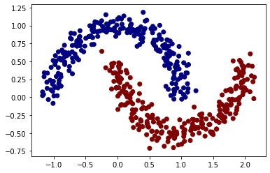
from sklearn.datasets import make_moons
X, y = make_moons(n_samples=500, noise=0.1)
y = y.reshape(-1, 1)
model_nn = Model(lr=0.0001, epochs=1000)
model_nn.add(Layer(2, 'relu'))
model_nn.add(Layer(4, 'relu'))
model_nn.add(Layer(8, 'relu'))
model_nn.add(Layer(8, 'relu'))
model_nn.add(Layer(5, 'relu'))
model_nn.add(Layer(1, 'sigmoid'))
model_nn.fit(X, y)
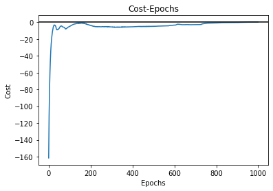
cost = model_nn.cost
plt.plot(range(len(cost)), cost)
plt.axhline(color='k')
plt.title("Cost-Epochs")
plt.xlabel('Epochs')
plt.ylabel('Cost')
We can also see how the cost changes as epoch increases:
Visualization the result by drawing decision boundary. In comparison, we also plot the result from MLP in sklearn with the same dataset:
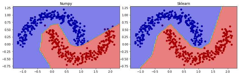
Not a bad job.
You can also review the code at
jupyter notebook code