
Preface
keras is a building-blocks-like package for deep learning and well-known for its flexibility. In This article, we will apply backpropagation and write a keras like MLP (multilayer perceptron) with numpy.
1. What is perceptron, how it works?
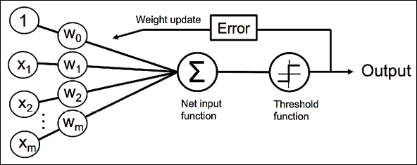
Before we get into MLP, we obviously need to understand what is perceptron. For simplicity, let’s consider a binary classification problem with a decision function $\phi(z)$ that has two possible outputs 1 and -1, representing class 1 and class 2 respectively, where $Z$ is a linear combination with input $x_i$ and corresponding weights $w_i$. Hence,
$Z = w_1x_1 + w_2x_2 + … + w_mx_m = sum_(i=1)^m w_ix_i$ or:
$W = [[W_1], […], [W_m]], X = [[X_1], […], [X_m]]$
if we add a bias term, $b$ to $Z$, or here for uniformity, we set $x_0 = 1$ and $w_0 = b$, we hence modify our formula as:
$Z = w_0x_0 + w_1x_1 + w_2x_2 + … + w_mx_m = sum_(i=0)^m w_ix_i = W^TX$
and our decision function:
$\phi(z) = {(1,ifz>=0,,,),(-1,otherwise,,,):}$
Next, we will do following steps to train a perceptron:
- Initialize the weighs to small random numbers, we here can use stand normal distribution to do so.
- For each training example, $x^(i)$:
2.1. Compute the output values $hat y$, the one from decision function $\phi(z)$
2.2. Update the weights by comparing to $y$ and $hat y$ to minimize the loss function 1
2.3. Repeat 2.2 for several times (epochs)
The process could be explained as follows:
Notice that if we:
- Drop the decision function $\phi(z)$, and use MSE (Mean Squared Error) as loss function, the perceptron will become to a linear regression (ordinary least square, more specifically)
- Use Sigmoid function to replace $\phi(z)$ and use Log loss (or called binary cross-entropy), the perceptron will become to a logistic regression
2. What is a MLP? How to apply backpropagation to train a MLP
Frankly speaking, multilayer perceptron is nothing more than a combination of multiple perceptron. Now, we (1) rename $\phi(z)$ as Activation Function, which provides model with ability to deal with nonlinear problems (recall Z is just a linear combination). (2) Connect each perceptron together to generate a new model.
we call the first and the last layer input and output layers respectively. The middle layers are called hidden layers.
A three layers MLP would be as follows:
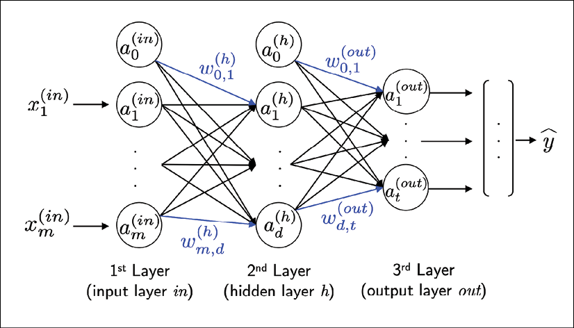
where $a_i^n$ is simply equal to $\phi(z)$ for convenience. Notice that the outputs of the previous layer are obviously the inputs of the next layer.
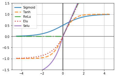
Also, Activation Functions are not necessarily the binary function showed above. Some common activation functions are, for example, Tanh, ReLU, Sigmoid, ELU, and SELU. Showed as the plot:
Similar to training a perceptron, we need to:
- Initialize the weighs to small random numbers, we here can use stand normal distribution to do so.
- For each training example, $x^(i)$:
2.1. Go through each layer (multiplied by its weights and applied to its activation function), until we come up with the final output $hat y$.
2.2. Update the weights by comparing to $y$ and $hat y$ to minimize the loss function
2.3. Repeat 2.1 and 2.2 for several times (epochs)
The process 2.1 is self-explained and called forward propagation. We next need to take a deep look at 2.2.
For a loss function(or cost function) $C_0$, if we update weights $W$ based on a rule that $W := W - lambda (delC_0)/(delW)$, where $lambda$ is called learning rate, we see the weights will be updated with a very small step every time until $(delC_0)/(delW) = 0$, which is the time we find the minimal value of the cost function relative to weights. This straightforward yet powerful algorithm is called Gradient Descent.
Basically, there are two variants for the Gradient Descent. If we update weights with all input samples, we call this algorithm Batch Gradient Descent or BGD. On the other hand, we can also randomly pick a subset of the input samples to update weights, this progress would result in a decline in the accuracy of each “step” (since it’s not the real $(delC_0)/(delW)$, but a subset of it), but this move will speed up our training processes dramatically. This variant is called Stochastic Gradient Descent or BGD.
Since $lambda$ (learning rate) is a hyperparameter that we manually set before the learning process, the only problem we have to handle is to find $(delC_0)/(delW)$.
According to the chain rule:
$(delC_0)/(delW^((L))) = (delZ^((L)))/(delW^((L))) (delA^((L)))/(delZ^((L))) (delC_0)/(delA^((L))) = A^((L-1))phi_z^’(delC_0)/(delA^((L)))$ $(1.1)$
, where $A^((L))$ meaning the result of activation function at layer $L$, and so on.
for the last term, $(delC_0)/(delA^((L)))$, because we can easily get the outcome of the output layer, we also need to know the $C_0$ derivative relative to $A^((L-1))$.
Hence:
$(delC_0)/(delA^((L-1))) = (delZ^((L)))/(delA^((L-1)))(delA^((L)))/(delZ^((L)))(delC_0)/(delA^((L))) = W^((L))phi_z^’(delC_0)/(delA^((L)))$ $(1.2)$
Similarly, with respect to bias term, $b$ (notice, for computational convenience, we split $b$ from $W$):
$(delC_0)/(delb^((L))) = (delZ^((L)))/(delb^((L))) (delA^((L)))/(delZ^((L))) (delC_0)/(delA^((L))) = 1phi_z^’(delC_0)/(delA^((L)))$ $(1.3)$
Finally, we can use a loop to calculate $(delC_0)/(delW)$ for each layer (from the last layer go back to the first) and to update weights based on Gradient Descent algorithm. We call this process Backpropagation.
We now understand the basic idea of MLP and training method. The next part will get started to code these processes.
-
We here will apply an approach called “Gradient Decent” to update weights. Since MLP and perceptron share the same method, we will explain it later. ↩